In finance, a price (premium) is paid or received for purchasing or selling options. This article discusses the calculation of this premium in general. For further detail, see: Mathematical finance § Derivatives pricing: the Q world for discussion of the mathematics; Financial engineering for the implementation; as well as Financial modeling § Quantitative finance generally.
Premium components
This price can be split into two components: intrinsic value, and time value (also called "extrinsic value").[1]
Intrinsic value
The intrinsic value is the difference between the underlying spot price and the strike price, to the extent that this is in favor of the option holder. For a call option, the option is in-the-money if the underlying spot price is higher than the strike price; then the intrinsic value is the underlying price minus the strike price. For a put option, the option is in-the-money if the strike price is higher than the underlying spot price; then the intrinsic value is the strike price minus the underlying spot price. Otherwise the intrinsic value is zero.
For example, when a DJI call (bullish/long) option is 18,000 and the underlying DJI Index is priced at $18,050 then there is a $50 advantage even if the option were to expire today. This $50 is the intrinsic value of the option.
In summary, intrinsic value:
- = current stock price − strike price (call option)
- = strike price − current stock price (put option)
Extrinsic (Time) value
The option premium is always greater than the intrinsic value up to the expiration event. This extra money is for the risk which the option writer/seller is undertaking. This is called the time value.
Time value is the amount the option trader is paying for a contract above its intrinsic value, with the belief that prior to expiration the contract value will increase because of a favourable change in the price of the underlying asset. The longer the length of time until the expiry of the contract, the greater the time value. So,
- Time value = option premium − intrinsic value
Other factors affecting premium
There are many factors which affect option premium. These factors affect the premium of the option with varying intensity. Some of these factors are listed here:
- Price of the underlying: Any fluctuation in the price of the underlying (stock/index/commodity) obviously has the largest effect on premium of an option contract. An increase in the underlying price increases the premium of call option and decreases the premium of put option. Reverse is true when underlying price decreases.
- Strike price: How far is the strike price from spot also affects option premium. Say, if NIFTY goes from 5000 to 5100 the premium of 5000 strike and of 5100 strike will change a lot compared to a contract with strike of 5500 or 4700.
- Volatility of underlying: Underlying security is a constantly changing entity. The degree by which its price fluctuates can be termed as volatility. So a share which fluctuates 5% on either side on daily basis is said to have more volatility than e.g. stable blue chip shares whose fluctuation is more benign at 2–3%. Volatility affects calls and puts alike. Higher volatility increases the option premium because of greater risk it brings to the seller.
- Payment of Dividend: Payment of Dividend does not have direct impact on value of derivatives but it does have indirect impact through stock price. We know that if dividend is paid, stock goes ex-dividend therefore price of stock will go down which will result into increase in Put premium and decrease in Call premium.
Apart from above, other factors like bond yield (or interest rate) also affect the premium. This is because the money invested by the seller can earn this risk free income in any case and hence while selling option; he has to earn more than this because of higher risk he is taking.
Pricing models
Because the values of option contracts depend on a number of different variables in addition to the value of the underlying asset, they are complex to value. There are many pricing models in use, although all essentially incorporate the concepts of rational pricing (i.e. risk neutrality), moneyness, option time value and put–call parity.
The valuation itself combines (1) a model of the behavior ("process") of the underlying price with (2) a mathematical method which returns the premium as a function of the assumed behavior.
The models in (1) range from the (prototypical) Black–Scholes model for equities, to the Heath–Jarrow–Morton framework for interest rates, to the Heston model where volatility itself is considered stochastic. See Asset pricing for a listing of the various models here.
As regards (2), the implementation, the most common approaches are:
- Closed form, analytic models: the most basic of these are the Black–Scholes formula and the Black model.
- Lattice models (Trees): Binomial options pricing model; Trinomial tree
- Monte Carlo methods for option pricing
- Finite difference methods for option pricing
- More recently, the volatility surface-aware models in the local volatility and stochastic volatility families.
The Black model extends Black-Scholes from equity to options on futures, bond options, swaptions, (i.e. options on swaps), and interest rate cap and floors (effectively options on the interest rate).
The final four are numerical methods, usually requiring sophisticated derivatives-software, or a numeric package such as MATLAB. For these, the result is calculated as follows, even if the numerics differ: (i) a risk-neutral distribution is built for the underlying price over time (for non-European options, at least at each exercise date) via the selected model, as calibrated to the market; (ii) the option's payoff-value is determined at each of these times, for each of these prices; (iii) the payoffs are discounted at the risk-free rate, and then averaged. For the analytic methods, these same are subsumed into a single probabilistic result; see Black–Scholes model § Interpretation.
Post crisis
After the financial crisis of 2007–2008, counterparty credit risk considerations were brought into the valuation, previously using the risk-free rate to discount the payoff. Here, there are [2] three major developments re option pricing:
- For discounting, the overnight indexed swap (OIS) curve is typically used for the "risk free rate", as opposed to LIBOR as previously; see Interest rate swap § Valuation and pricing. Relatedly, the "Multi-curve framework" is now standard in the valuation of interest rate derivatives and for fixed income analysis more generally.
- To ensure that option prices are consistent with the volatility surface, the numerics will incorporate a zeroth calibration step, such that observed prices are returned before new prices and / or "greeks" can be calculated. To do so, banks will apply local- or stochastic volatility models, such as Heston mentioned above (or less common, implied trees).
- The risk neutral value, no matter how determined, is adjusted for the impact of counterparty credit risk via a credit valuation adjustment, or CVA, as well as various of the other XVA which may also be appended.
References
- ^ "Extrinsic Value Definition | Britannica Money". www.britannica.com. Retrieved 2023-05-09.
- ^ Derivatives Pricing after the 2007-2008 Crisis: How the Crisis Changed the Pricing Approach, Didier Kouokap Youmbi, Bank of England – Prudential Regulation Authority
The Heston Model and its Extensions in Matlab and C#:
Fabrice D. Rouah, with Foreword by Steven L. Heston -
Tap into the power of the most popular stochastic volatility model for pricing equity derivatives.
C# for Financial Markets:
Andrea Germani - Daniel Duffy
A practice-oriented guide to using C# to design and program pricing and trading models.
Practical C# and WPF for Financial Markets:
Advanced C#, WPF, and MVVM Programming for Quant Developers/Analysts and Individual Traders
Jack Xu -
Practical C# and WPF for Financial Markets provides a complete explanation of .NET programming in quantitative finance.
Practical Quantitative Finance with ASP.NET Core and Angular:
Building Ultra-Modern, Responsive Single-Page Web Applications for Quantitative Finance using ASP.NET Core and Angular.
Jack Xu -
Building Ultra-Modern, Responsive Single-Page Web Applications for Quantitative Finance using ASP.NET Core and Angular.
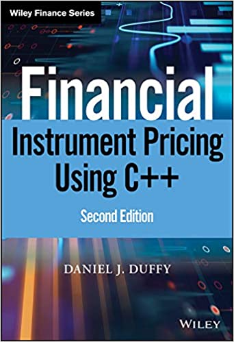
Financial Instrument Pricing Using C++ 2nd Ed.:
- Daniel Duffy
This complete guide to C++ and computational finance is a major extension to Daniel J. Duffy's 2004 edition.
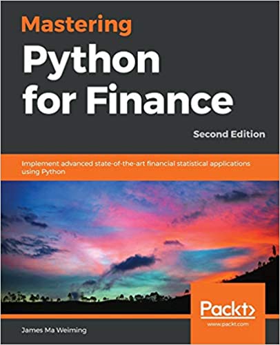
Mastering Python for Finance:
Implement advanced state-of-the-art financial statistical applications using Python, 2nd Edition
James Ma Weiming -
Explore advanced financial models, build state-of-the-art infrastructure, empower your financial applications.
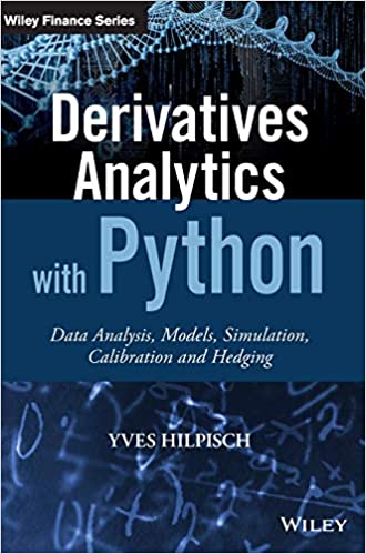
Derivatives Analytics with Python:
Data Analysis, Models, Simulation, Calibration and Hedging
- Yves Hilpisch
This book is the finance professional's guide to exploiting Python's capabilities for efficient and performing derivatives analytics.
Financial Modelling: Theory, Implementation and Practice with MATLAB Source:
Daniel Wetterau - Jörg Kienitz
A unique contribution to the application of quantitative techniques to financial problems and programming using Matlab.
Options and Derivatives Programming in C++20:
Algorithms and Programming Techniques for the Financial Industry
Carlos Oliveira -
Master the features of C++ that are frequently used to write financial software for options and derivatives, including the STL, templates, functional programming, and numerical libraries.
Quantitative Finance (Statistics in Practice):
Maria C. Mariani and Ionut Florescu -
This book presents quantitative finance theory through applications to specific practical problems and comes with accompanying coding techniques in R and MATLAB.
Quantitative Finance: An Object-Oriented Approach in C++:
Erik Schlögl -
Providing readers with a foundation in the key methods and models of quantitative finance. Keeping the material as self-contained as possible, the author introduces computational finance with a focus on practical implementation in C++.

